Calculating and plotting VOD

import gnssvod as gv
import pandas as pd
import matplotlib.pyplot as plt
from matplotlib.collections import PatchCollection
import matplotlib.dates as mdates

calc_vod()

The first step is to calculate VOD for different bands.

One problem is that the observations labels (‘S1C’,’S1X’, etc.) are not always associated to the same frequency depending on which constellation is observed. The labeling also changes according to the RINEX versions.

The calc_vod() function calculates VOD by first evaluating the SNR difference between the individual pairs of observations. The SNR from the clear-sky reference is subtracted from the SNR at the subcanopy station. The attenuation is corrected for the elevation of the satellite, yielding a VOD value.

# set which data files should be loaded
pattern = 'data_RINEX3.03/Laeg_paired/nc/*.nc'
# define how to associate stations together. Always put reference station first.
pairings = {'Laeg':('CH-Laeg_ref','CH-Laeg_grn')}
# define if some observables with similar frequencies should be combined together. In the future, this should be replaced by the selection of frequency bands.
bands = {'VOD1':['S1','S1X','S1C'],'VOD7':['S7','S7X','S7C']}

vod = gv.calc_vod(pattern,pairings,bands)
vod = vod['Laeg']
vod

		VOD1	VOD7	Azimuth	Elevation
Epoch	SV
2023-08-01 00:07:45	C19	NaN	NaN	-97.0	26.1
	C20	NaN	NaN	-144.2	10.6
	C23	NaN	NaN	97.5	3.1
	C27	NaN	NaN	153.1	29.2
	C28	NaN	NaN	92.9	42.9
...	...	...	...	...	...
2023-08-09 23:59:45	R14	2.327782	NaN	-42.8	57.4
	R23	NaN	NaN	NaN	NaN
	R24	-0.010382	NaN	149.7	26.8
	S23	NaN	NaN	NaN	NaN
	S36	NaN	NaN	NaN	NaN

1495088 rows × 4 columns

Hemispheric plot of VOD

Same as in the previous example, we will use the Hemi class to calculate and plot a gridded representation of VOD

# intialize hemispheric grid
hemi = gv.hemibuild(2)
# get patches for plotting later
patches = hemi.patches()
# classify vod into grid cells, drop azimuth and elevation afterwards as we don't need it anymore
vod = hemi.add_CellID(vod).drop(columns=['Azimuth','Elevation'])
# get average value per grid cell
vod_avg = vod.groupby(['CellID']).agg(['mean', 'std', 'count'])
# flatten the columns
vod_avg.columns = ["_".join(x) for x in vod_avg.columns.to_flat_index()]
vod_avg

	VOD1_mean	VOD1_std	VOD1_count	VOD7_mean	VOD7_std	VOD7_count
CellID
0	0.879183	0.507725	184	1.810452	0.509661	57
1	0.757022	0.561797	374	1.330002	0.449482	120
2	0.572596	0.531027	158	2.221168	0.778867	70
3	2.128975	1.155671	58	1.266589	0.548697	58
4	0.834365	0.637610	39	0.907239	0.424226	39
...	...	...	...	...	...	...
6420	0.020885	0.019975	26	0.034187	0.015323	26
6431	1.572118	1.512187	37	NaN	NaN	0
6432	0.086603	0.033302	18	NaN	NaN	0
6438	0.070679	0.056207	32	NaN	NaN	0
6439	0.039912	0.015835	8	NaN	NaN	0

5124 rows × 6 columns

fig, ax = plt.subplots(1,2,figsize=(17,14),subplot_kw=dict(projection='polar'))

vod_names = ['VOD1','VOD7']
for i, iname in enumerate(vod_names):
    # associate the mean values to the patches, join inner will drop patches with no data, making plotting slightly faster
    ipatches = pd.concat([patches,vod_avg[f"{iname}_mean"]],join='inner',axis=1)
    # plotting with colored patches
    pc = PatchCollection(ipatches.Patches,array=ipatches[f"{iname}_mean"],edgecolor='face', linewidth=1)
    pc.set_clim([-0.1,3])
    ax[i].add_collection(pc)
    ax[i].set_rlim([0,90])
    ax[i].set_theta_zero_location("N")
    ax[i].set_theta_direction(-1)
    ax[i].set_title(iname)

plt.colorbar(pc, ax=ax, location='bottom', shrink=.5, pad=0.05, label='GNSS-VOD')

<matplotlib.colorbar.Colorbar at 0x7f772615c520>

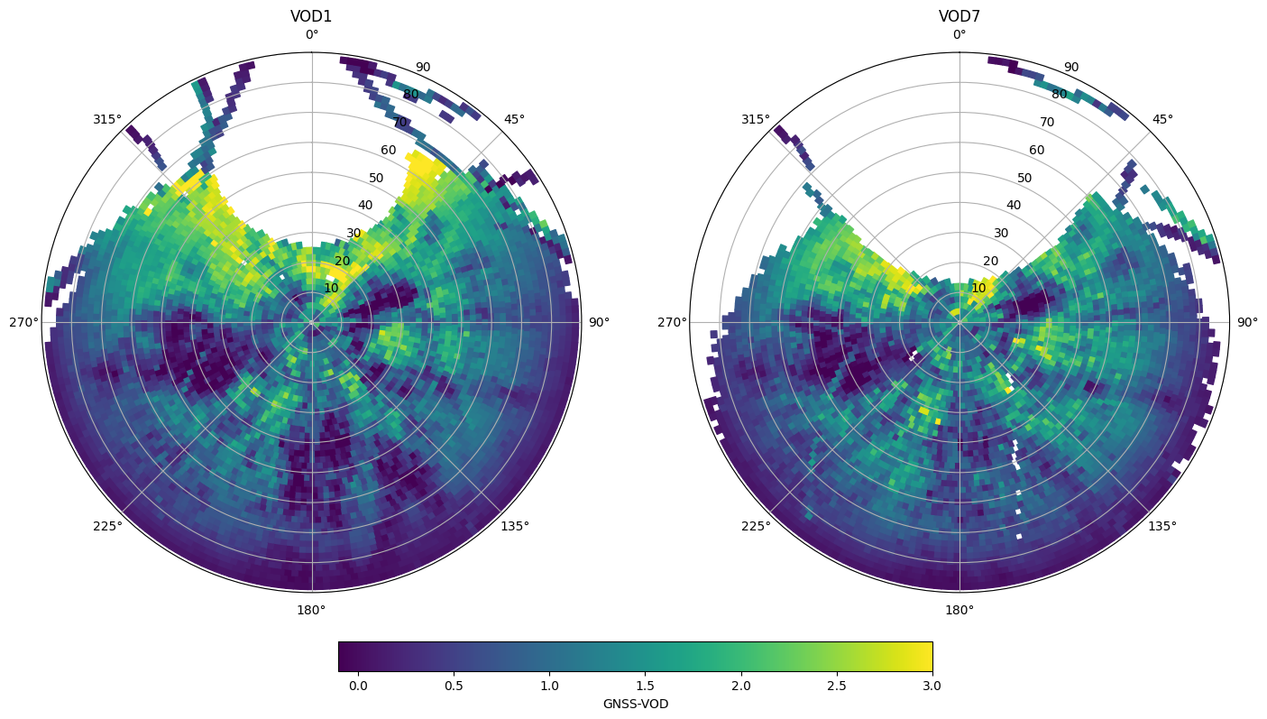
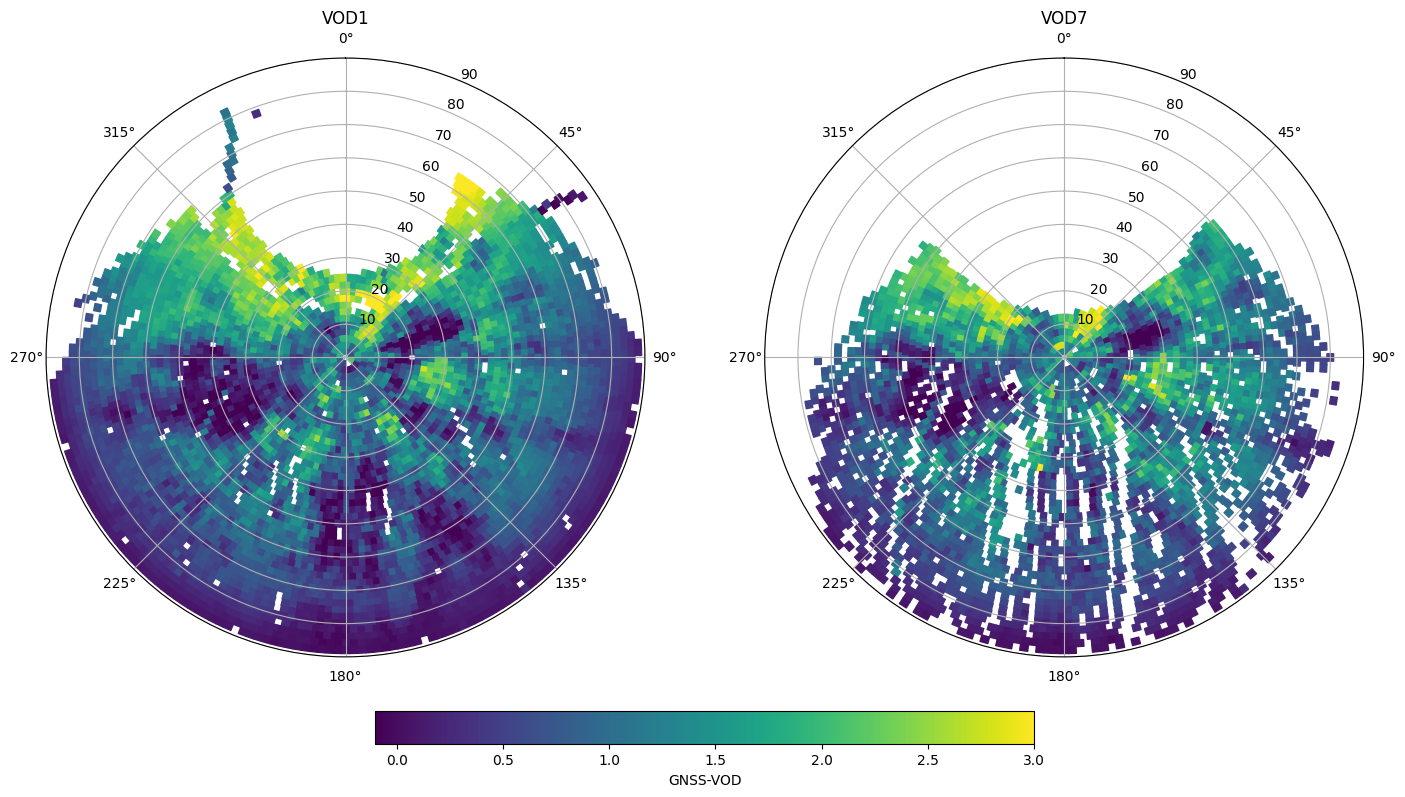
It can be a good idea to only plot the average if a minimum number of values were used to calculate an average. Sometimes results at the edges are only based on a few data points and are not very reliable.

fig, ax = plt.subplots(1,2,figsize=(17,14),subplot_kw=dict(projection='polar'))

vod_names = ['VOD1','VOD7']
for i, iname in enumerate(vod_names):
    # associate the mean values to the patches, join inner will drop patches with no data, making plotting slightly faster
    ivod_data = vod_avg[f"{iname}_mean"].where(vod_avg[f"{iname}_count"]>40)
    ipatches = pd.concat([patches,ivod_data],join='inner',axis=1)
    # plotting with colored patches
    pc = PatchCollection(ipatches.Patches,array=ipatches[f"{iname}_mean"],edgecolor='face', linewidth=1)
    pc.set_clim([-0.1,3])
    ax[i].add_collection(pc)
    ax[i].set_rlim([0,90])
    ax[i].set_theta_zero_location("N")
    ax[i].set_theta_direction(-1)
    ax[i].set_title(iname)

plt.colorbar(pc, ax=ax, location='bottom', shrink=.5, pad=0.05, label='GNSS-VOD')

<matplotlib.colorbar.Colorbar at 0x7f7725ba6df0>

Calculation of VOD time series

Because the tracks of the satellites are not random but tend to repeat every day, one has to be a bit careful when computing temporal averages of VOD. For instance, satellites of the GPS constellation repeat twice every sidereal day (1 sidereal day = 23h 56m 4s). Other constellations (below) have slightly more complex repeat times.

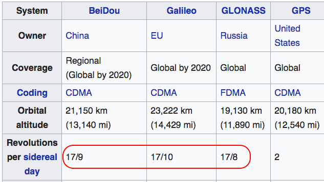
Imagine what would happen if most GNSS satellites happen to repeatedly go over slightly denser areas of the canopy every day at around 3:30pm. We would tend to see a peak in VOD each day at that time. However, the average VOD of the forest is not actually increasing, the peak exists only because we happen to be measuring parts of the canopy that are on average slightly denser. Especially when looking at very small changes in VOD (for instance diurnal variability), these repeating orbits create spurious signals and obfuscate the real variability. Check Humphrey & Frankenberg 2023, Figure 7 to see how this affects time series.

Processing a more accurate VOD time series involves three steps:

• Calculating a baseline (long-term mean) hemispheric VOD over a sufficiently long time period (which we just did)

• Calculate VOD anomalies by subtracting the baseline from each instantaneous VOD measurement

• Calculate a time series based on the VOD anomalies

Calculating VOD anomalies

Here we merge back the VOD average to the original dataframe.

# merge statistics with the original VOD measurements
vod_anom = vod.join(vod_avg,on='CellID')
vod_anom

		VOD1	VOD7	CellID	VOD1_mean	VOD1_std	VOD1_count	VOD7_mean	VOD7_std	VOD7_count
Epoch	SV
2023-08-01 00:07:45	C19	NaN	NaN	3733	0.485518	0.242357	208	0.753132	0.240639	58
	C20	NaN	NaN	5444	0.416537	0.147121	102	0.385905	0.158380	62
	C23	NaN	NaN	6052	0.250855	0.050505	183	NaN	NaN	0
	C27	NaN	NaN	3267	0.051724	0.334082	54	0.867515	0.387465	38
	C28	NaN	NaN	2130	1.501628	0.634895	250	1.260002	0.435578	71
...	...	...	...	...	...	...	...	...	...	...
2023-08-09 23:59:45	R04	1.116509	NaN	3128	0.541466	0.430518	406	0.899058	0.428780	79
	R12	0.274069	NaN	6048	0.295512	0.070216	190	NaN	NaN	0
	R13	2.020736	NaN	1795	1.501337	0.760002	462	1.455787	0.513682	62
	R14	2.327782	NaN	1044	2.584283	0.825547	198	NaN	NaN	0
	R24	-0.010382	NaN	3668	-0.022531	0.266441	200	0.552734	0.203059	95

1329259 rows × 9 columns

Anomalies are simply obtained with:

vod_anom['VOD1_anom'] = vod_anom['VOD1']-vod_anom['VOD1_mean']
vod_anom['VOD7_anom'] = vod_anom['VOD7']-vod_anom['VOD7_mean']

Calculating the anomaly time series

Here we calculate an hourly average

vod_ts = vod_anom.groupby(pd.Grouper(freq='1h', level='Epoch')).mean()
vod_ts

	VOD1	VOD7	CellID	VOD1_mean	VOD1_std	VOD1_count	VOD7_mean	VOD7_std	VOD7_count	VOD1_anom	VOD7_anom
Epoch
2023-08-01 00:00:00	1.045700	0.857200	3161.386060	1.000563	0.432741	298.288867	0.975316	0.368189	67.404259	-0.014699	0.028733
2023-08-01 01:00:00	1.097543	0.906498	3125.360222	1.068297	0.440577	298.365611	1.010482	0.369235	76.660843	-0.007610	-0.021655
2023-08-01 02:00:00	1.007393	1.047247	3176.665345	0.988260	0.426496	286.419311	0.986190	0.358648	70.151769	-0.034646	0.010036
2023-08-01 03:00:00	0.969277	1.096157	2696.083424	1.026343	0.484076	331.838911	1.086580	0.405147	85.611051	0.004872	-0.000651
2023-08-01 04:00:00	1.104497	1.075735	2315.294587	1.080343	0.523946	336.100631	1.030475	0.411516	84.555629	0.024695	0.018333
...	...	...	...	...	...	...	...	...	...	...	...
2023-08-09 19:00:00	1.148011	1.177217	2475.636711	1.151665	0.518803	352.278738	1.122829	0.416244	81.463123	-0.020028	-0.066742
2023-08-09 20:00:00	0.987982	1.222887	2506.069470	1.025942	0.484028	321.785275	1.046329	0.407231	77.058833	-0.023637	-0.028753
2023-08-09 21:00:00	1.132818	1.001172	2610.778375	1.093195	0.537218	270.739590	1.073045	0.405216	68.214070	-0.051414	-0.114403
2023-08-09 22:00:00	0.941130	0.924344	2945.734087	0.920403	0.465508	295.216509	0.927142	0.354828	80.147437	0.014564	-0.033115
2023-08-09 23:00:00	0.922004	0.900242	2964.178333	0.969349	0.451153	317.742046	0.997615	0.381067	79.576440	-0.017199	-0.023575

216 rows × 11 columns

We should not forget to add the mean VOD back, otherwise the anomaly time series will be centred around zero

vod_ts['VOD1_anom'] = vod_ts['VOD1_anom']+vod_ts['VOD1'].mean()
vod_ts['VOD7_anom'] = vod_ts['VOD7_anom']+vod_ts['VOD7'].mean()

Now let’s compare our time series, with and without subtracting the baseline.

vod_names = ['VOD1','VOD1_anom']

fig, ax = plt.subplots(1,figsize=(10,5))
for i, iname in enumerate(vod_names): 
    # plot each measurement and color by signal to noise ratio
    hs = ax.plot(vod_ts.index.get_level_values('Epoch'),vod_ts[iname],label=iname)
    
myFmt = mdates.DateFormatter('%d-%b')
ax.xaxis.set_major_formatter(myFmt)
ax.set_ylabel('GNSS-VOD (L1)')
ax.legend()
plt.title('GNSS-VOD at Lägeren Tower (CH-Laeg, Switzerland), August 2023')
plt.savefig('figures/illustration_vod.png',facecolor='white', transparent=False,bbox_inches='tight')

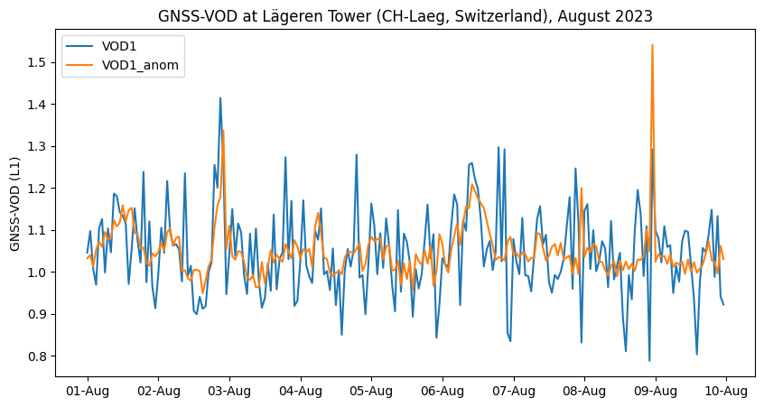
We clearly see how subtracting the gridded hemispheric average before calculating the time series has substantially reduced the noise in our VOD time series. Here we see short spikes usually corresponding to rain events and water interception by the canopy. A very small diurnal cycle is somewhat visible on August 3 to 6, with dehydration during day and rehydration overnight.

Longer time series

In principle, when calculating a time series over several months, the baseline should be regularly updated. One option could be to go for a “moving” baseline, with a window of a few weeks.

In the next release, there should be some functions to do exactly that with a batch logic (i.e. automatically).